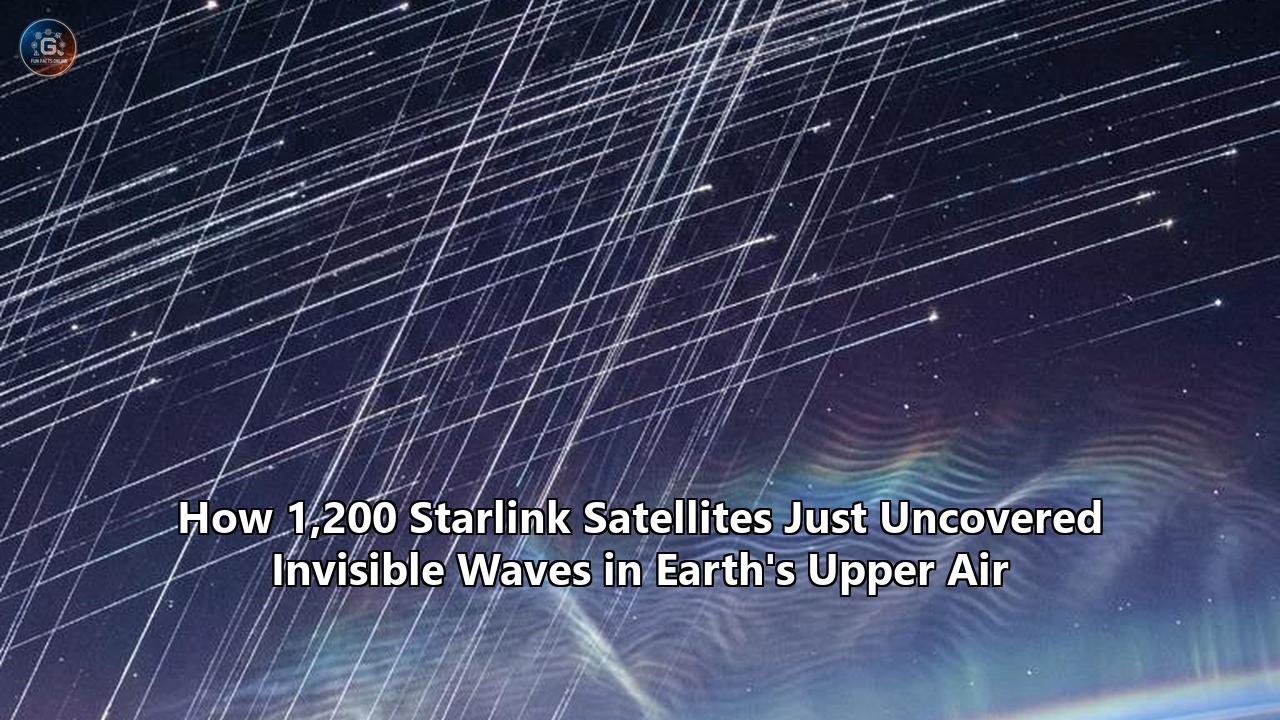
An orbital fleet launched to deliver high-speed broadband has unexpectedly solved one of the most stubborn observational challenges in space physics. By analyzing minute variations in the trajectories of roughly 1,200 Starlink satellites operating in low Earth orbit, researchers at Kyoto University have created the first two-dimensional tomographic maps of neutral density ripples and traveling disturbances in the thermosphere.
The study, led by space physicist Mamoru Yamamoto at Kyoto University's Research Institute for Sustainable Humanosphere and published in Earth, Planets and Space, demonstrates that commercial mega-constellations can double as an unintended, planet-scale scientific instrument. By converting orbital drag data into precise atmospheric density fields, the researchers detected sweeping, previously unresolvable fluctuations at altitudes of 482 kilometers (roughly 300 miles) above the planet's surface.
                     SOLAR WIND & JOULE HEATING
                                │
                                ▼
  ┌──────────────────────────────────────────────────────────────┐
  │         THERMOSPHERE (100–1000 km) [99% Neutral Gas]         │
  │                                                              │
  │   (~482 km Shell)   🛰️       🛰️       🛰️       🛰️       🛰️     │
  │   1,200 Starlink ───► Drag ──► Orbital Energy Loss (ΔE)     │
  │   Satellites                  │                              │
  │                               ▼                              │
  │                  Inverse Tomographic Mapping                 │
  │                  & Spherical Harmonics Matrix                │
  │                               │                              │
  │                               ▼                              │
  │                 2D Map of Invisible Density                  │
  │                 Waves & Traveling Disturbances               │
  └───────────────────────────────┬──────────────────────────────┘
                                  │ Cross-Validation (Ratio: 0.95)
                                  ▼
  ┌──────────────────────────────────────────────────────────────┐
  │            ESA SWARM A & B In-Situ Benchmark                 │
  └──────────────────────────────────────────────────────────────┘
The breakthrough represents the culmination of a four-year escalation that began with an orbital disaster, progressed through mathematical adaptations borrowed from clinical radiology, and ended with a verification against European Space Agency (ESA) research satellites. The data reveals that Earth's upper air is far from a serene vacuum; it is a turbulent, undulating medium driven by solar energy, geomagnetic storms, and energy rising from weather systems lower down.
1. The 99-Percent Blindspot: Why the Upper Atmosphere Kept Its Secrets
To understand how 1,200 commercial satellites solved this problem, it is necessary to examine the physics of the atmospheric layer extending between 100 and 1,000 kilometers above sea level: the thermosphere.
Layer Altitude        Atmospheric Composition & Sensing Profile
───────────────────────────────────────────────────────────────────────────
Exosphere             Exobase to ~10,000 km | Pure hydrogen/helium, ballistic escape
───────────────────────────────────────────────────────────────────────────
Thermosphere          100 km to ~1,000 km   | 99% Neutral Gas (N2, O, O2)
                      (Starlink @ 482 km)   | [Historically Blind to Radar/Radio]
                                            | 1% Ionized Plasma (Ionosphere)
                                            | [Trackable via GPS Phase Delays]
───────────────────────────────────────────────────────────────────────────
Mesosphere            50 km to 100 km       | Middle atmosphere, meteor ablation
───────────────────────────────────────────────────────────────────────────
Stratosphere          12 km to 50 km        | Ozone layer, balloon sounding ceiling
───────────────────────────────────────────────────────────────────────────
Troposphere           Surface to 12 km      | Weather systems, dense meteorological net
For over six decades, atmospheric scientists have contended with an observational divide at the boundary of space. More than 99 percent of the gas in the thermosphere is electrically neutral, consisting primarily of atomic oxygen ($\text{O}$), molecular nitrogen ($\text{N}_2$), and molecular oxygen ($\text{O}_2$). The remaining fraction—less than one percent—is ionized into charged electrons and positive ions by solar extreme ultraviolet (EUV) and X-ray radiation, forming the overlapping ionosphere.
Because charged particles refract, disperse, and delay electromagnetic signals, the ionosphere is comparatively easy to measure. Ground-based ionosondes, incoherent scatter radars, and terrestrial Global Navigation Satellite System (GNSS) receivers tracking total electron content (TEC) have long provided real-time diagnostic coverage of ionospheric weather.
The neutral thermosphere, however, offers no such convenience. It does not interact with low-frequency radio waves, remains invisible to weather radar, and is situated far too high for weather balloons (which pop below 40 km) or research aircraft. Sounding rockets pass through it in minutes, providing only fleeting vertical profiles.
Pencil-Beam Satellite Track (CHAMP / GOCE / SWARM):
Orbit 1 ─────────► [Single 1D Track]
                     (No simultaneous longitudinal or latitudinal width)

Mega-Constellation Tomography (1,200 Starlink Nodes):
Orbit 1  ═══════════════════════════════════════════════►
Orbit 2    ═══════════════════════════════════════════════►   [Simultaneous 2D
Orbit 3      ═══════════════════════════════════════════════►  Global Dynamic
Orbit ...      ═══════════════════════════════════════════════► Mesh]
Orbit N          ═══════════════════════════════════════════════►
For decades, direct measurements of neutral thermospheric density relied on a handful of specialized scientific spacecraft equipped with electrostatic accelerometers or precision tracking systems, including:
- The German Aerospace Center’s CHAMP mission (2000–2010)
- The NASA/German GRACE tandem (2002–2017)
- The European Space Agency’s GOCE spacecraft (2009–2013)
- ESA’s three-satellite SWARM constellation (2013–present)
While these missions produced exquisite in-situ measurements, they suffered from a fundamental geometric constraint: they were 1D single-point probes. A solitary satellite flies along an orbital track like a weather sensor attached to a high-speed bullet train. It measures conditions directly along its flight path, but it cannot tell researchers what is occurring 500 kilometers to its left, 1,000 kilometers to its right, or how a dynamic wave front is propagating across global longitudes simultaneously.
As a result, theoretical atmospheric models like NRLMSIS (Naval Research Laboratory Mass Spectrometer and Incoherent Scatter Radar) had to rely on time-averaged climatological empirical formulas. They modeled the upper atmosphere as a smooth, predictable envelope that slowly swelled under sunlight and contracted at night. They had no way to capture localized, high-frequency density ripples.
2. February 2022: The 40-Satellite Wake-Up Call
The limitation of empirical models shifted from an academic inconvenience to an operational emergency on February 3, 2022.
SpaceX launched Falcon 9 flight Group 4-7 from Launch Complex 39A at Kennedy Space Center in Florida, carrying 49 Starlink satellites into an initial elliptical injection orbit with a perigee of roughly 210 kilometers. Deploying at this low altitude was a deliberate safety feature: if any spacecraft malfunctioned during early checkout, atmospheric drag would pull it down within days, preventing dead satellites from cluttering low Earth orbit.
Timeline of the February 2022 Starlink Loss:
──────────────────────────────────────────────────────────────────────────
Feb 3, 2022 (Launch)    Falcon 9 deploys 49 Starlink satellites at ~210 km
Feb 3–4, 2022 (Storm)   M-class solar flare CME triggers G1 geomagnetic storm
Feb 4, 2022 (Impact)    Joule heating expands thermosphere; drag spikes up to +137%
Feb 4–5, 2022 (Maneuver)SpaceX puts satellites in "edge-on" low-drag safe mode
Feb 5–7, 2022 (Reentry) Up to 40 satellites stall, lose altitude, and burn up
Shortly after deployment, a coronal mass ejection (CME) from an M-class solar flare struck Earth's magnetosphere. The geomagnetic disturbance was modest, registering as a minor G1-class storm on the NOAA space weather scale. Ground-based space weather models predicted standard operational parameters.
Reality inside the thermosphere was drastically different.
The incoming stream of charged solar plasma generated field-aligned electric currents that surged into Earth's auroral zones. This electrical energy drove intense Joule heating, dumping gigawatts of thermal power into the upper atmosphere. The air heated, expanded vertically, and formed large-scale traveling atmospheric disturbances (TADs)—massive acoustic-gravity wave crests that rippled equatorward at supersonic speeds.
           SOLAR CORONAL MASS EJECTION (CME)
                           │
                           ▼
             EARTH'S MAGNETOSPHERE
                           │
               (Field-Aligned Currents)
                           ▼
          AURORAL JOULE & PARTICLE HEATING
                           │
                           ▼
 ┌──────────────────────────────────────────────────┐
 │ THERMOSPHERIC EXPANSION & DENSITY SURGE (+137%)  │
 └─────────────────────────┬────────────────────────┘
                           │
             (Traveling Atmospheric Waves)
                           ▼
 ┌──────────────────────────────────────────────────┐
 │ SPACEX INJECTION ORBIT (210 km)                  │
 │ • Atmospheric drag overcomes ion thrusters       │
 │ • Satellites unable to raise orbits              │
 │ • 38–40 spacecraft burn up over the Caribbean    │
 └──────────────────────────────────────────────────┘
At the 210-kilometer injection altitude, atmospheric density did not rise incrementally; it surged. Drag on the newly deployed Starlink satellites increased by up to 50 to 137 percent above baseline levels.
SpaceX flight controllers ordered the satellites into a protective "edge-on" orientation, flying them like knives through the wind to minimize their cross-sectional area and reduce drag. The ion thrusters could not overcome the sudden, thick atmospheric waves. The spacecraft lost orbital velocity, stalled, and began falling. Over the next three days, 38 to 40 of the 49 satellites plunged into the lower atmosphere and disintegrated over the Caribbean Sea and Atlantic Ocean.
The 2022 incident exposed a dangerous reality: Earth's thermosphere is subject to sudden, wave-driven density surges that modern space tracking systems could neither forecast nor observe in real time. The incident made it clear that satellite operators could no longer treat the upper atmosphere as a static backdrop.
3. The Ephemeris Pivot: Turning Orbit Data into Sensors
In the aftermath of the 2022 storm, space tracking underwent a major operational evolution. SpaceX, operating thousands of active Starlink satellites in low Earth orbit, accelerated the public release of its orbital ephemeris data.
Historically, orbital analysts and civil trackers relied on Two-Line Element sets (TLEs) generated by the U.S. Space Force’s 18th Space Defense Squadron. While TLEs provide an overview of a satellite's orbit, they suffer from coarse temporal resolution and mathematical approximations that obscure minute, short-period aerodynamic variations.
Tracking Method Comparison:
──────────────────────────────────────────────────────────────────────────
Parameter            Two-Line Elements (TLE)    Starlink Ephemerides
──────────────────────────────────────────────────────────────────────────
Update Cadence       Once every 8 to 24 hours   Refreshed every 8 hours
Temporal Sampling    Single averaged epoch      1-minute position/velocity
Position Accuracy    ~1,000 meters              < 10–50 meters
Velocity Precision   Approximated Mean Motion   Precise 3-axis state vectors
Atmospheric Utility  Crude, 1D historical drag  Resolves high-frequency waves
──────────────────────────────────────────────────────────────────────────
SpaceX began publishing high-precision ephemerides refreshed every eight hours, detailing the precise position and velocity vectors of its constellation at one-minute intervals over a forward-looking 72-hour window.
At Kyoto University, Mamoru Yamamoto recognized an overlooked opportunity. Rather than treating atmospheric drag as a hazard or noise to be filtered out, that drag could be used as an environmental sensor.
                       SATELLITE TRAJECTORY TELEMETRY
                                     │
                                     ▼
        ┌─────────────────────────────────────────────────────────┐
        │  Calculate Total Mechanical Energy (Kinetic + Grav.)    │
        │             E_mech = (1/2) * m * v² + U_grav            │
        └────────────────────────────┬────────────────────────────┘
                                     │
                                     ▼
        ┌─────────────────────────────────────────────────────────┐
        │  Determine Energy Loss Rate (dE/dt) Over Orbital Arcs   │
        └────────────────────────────┬────────────────────────────┘
                                     │
                        Maneuver Detection Gate
                     ┌───────────────┴───────────────┐
                     ▼                               ▼
        ┌─────────────────────────┐     ┌─────────────────────────┐
        │ Active Thruster Firing  │     │ Non-Conservative Drag   │
        │ (Krypton/Argon Burn)    │     │      Force Detected     │
        │ [~80% Data Discarded]   │     └────────────┬────────────┘
        └─────────────────────────┘                  │
                                                     ▼
                                        ┌─────────────────────────┐
                                        │ Derive Neutral Density  │
                                        │    Around Satellite     │
                                        └─────────────────────────┘
Because every satellite traveling through the thermosphere collides with ambient neutral atoms and molecules, it constantly loses mechanical energy to aerodynamic resistance. The rate of that energy loss is directly proportional to the local air density.
The equation governing aerodynamic drag force ($F_D$) acting on a satellite is:
$$F_D = \frac{1}{2} \rho v_{\text{rel}}^2 C_D A$$
Where:
- $\rho$ is the neutral mass density of the thermosphere
- $v_{\text{rel}}$ is the velocity of the satellite relative to the co-rotating atmosphere
- $C_D$ is the aerodynamic drag coefficient
- $A$ is the effective cross-sectional area facing the ram direction
By rearranging the orbital energy conservation equations and tracking the rate of orbital mechanical energy decay ($\Delta E$) along a satellite’s flight path, scientists can calculate the ambient density ($\rho$) through which the satellite passed:
$$\Delta E = \int_{\text{orbit}} \mathbf{F}_D \cdot \mathbf{v} \, dt$$
The initial challenge, published by Yamamoto and colleague Takuya Sori in early 2026, relied on older TLE data. That preliminary test confirmed the core physics: drag trends tracked seasonal and solar-cycle shifts. But TLE datasets were too coarse to capture horizontal spatial structures or isolate localized atmospheric disturbances. To map upper-air waves, the researchers needed higher temporal resolution, greater spatial density, and a more advanced mathematical framework.
4. The Mathematical Breakthrough: Medical Tomography Pointed Skyward
By mid-2026, Yamamoto’s team moved from TLE tracking to SpaceX’s raw ephemerides. They targeted a single, highly populated orbital shell: approximately 1,200 first-generation Starlink satellites operating at an average altitude of 482 kilometers with an orbital inclination of 53 degrees.
Starlink Orbital Shell Parameters (Study Configuration):
• Active Satellites Analyzed: ~1,200 spacecraft
• Nominal Orbital Altitude:   482 kilometers
• Orbital Inclination:        53.0 degrees
• Ephemeris Sampling Rate:    1 data point per minute
• Orbit Reconstruction Span:  September 1–7, 2025
• Global Independent Tests:   19 distinct spatial runs
Moving from simple tracking to mapping dynamic atmospheric structures required overcoming two major technical obstacles:
The Thruster Maneuver Problem
Starlink satellites are not passive debris; they constantly fire onboard krypton and argon ion thrusters to adjust orbits, dodge space junk, maintain orbital phasing, and counter drag.
When analyzing the first dataset, the Kyoto team found active maneuvers in roughly 80 percent of satellite trajectories. If a thruster fires, the satellite's orbital energy jumps or stabilizes, disguising or mimicking atmospheric drag.
The researchers developed an automated maneuver-detection filter based on mean orbital elements. Any orbital arc exhibiting deliberate acceleration was isolated and removed, leaving only the clean, unpowered orbital decay driven solely by atmospheric drag.
           Ephemeris Trajectory Arc (1-min Cadence)
                              │
                              ▼
        ┌───────────────────────────────────────────┐
        │  Calculate Rate of Change of Semi-Major   │
        │             Axis: da/dt                   │
        └─────────────────────┬─────────────────────┘
                              │
               Exceeds Natural Drag Threshold?
               ┌──────────────┴──────────────┐
              YES                            NO
               ▼                             ▼
   ┌───────────────────────┐     ┌───────────────────────┐
   │ Manifold Thruster     │     │ Pure Aerodynamic Drag │
   │ Firing Identified     │     │ Path Confirmed        │
   │ [Reject from Inversion│     │ [Feed into Tomographic│
   │  Matrix]              │     │  Inversion Algorithm] │
   └───────────────────────┘     └───────────────────────┘
The Multi-Angle Inversion (Tomography)
The second obstacle was transforming hundreds of intersecting, one-dimensional satellite tracks into a coherent, two-dimensional map across latitude and longitude.
Yamamoto turned to tomography—the mathematical technique behind medical CT (computed tomography) scans. In a hospital CT scanner, X-ray beams pass through the human body from hundreds of rotating angles. By calculating how much each beam attenuates along its path, a computer solves an inverse matrix equation to reconstruct a high-resolution, three-dimensional cross-section of internal organs.
       Medical CT Scan vs. Thermospheric Orbital Tomography
──────────────────────────────────────────────────────────────────────────
Component            Hospital CT Scanner       Starlink Constellation
──────────────────────────────────────────────────────────────────────────
Sensing Ray          X-Ray Photon Beam         Satellite Orbital Arc
Medium Probed        Human Tissue / Bone       Neutral Thermosphere (482 km)
Measurement          Radiation Attenuation     Orbital Drag Energy Loss (ΔE)
Inverse Model        Radon Transform           Spherical Harmonics Inversion
Resulting Output     Cross-Sectional Organ     2D Global Map of Dynamic
                     Density Profile           Atmospheric Density Waves
──────────────────────────────────────────────────────────────────────────
In Yamamoto's formulation, the satellite is the probe, the upper atmosphere is the body, and the loss of orbital energy is the attenuation.
Because approximately 1,200 satellites crisscross each other across latitude and longitude bands between $53^\circ\text{N}$ and $53^\circ\text{S}$, their flight paths form a dense, woven lattice of intersecting trajectories.
By defining the global atmospheric density as a series of spherical harmonic expansion functions and applying an inverse matrix algorithm, the Kyoto team reconstructed a continuous 2D horizontal density field at an altitude of 482 kilometers.
For the first time, researchers had a mathematical framework capable of isolating Starlink satellites atmospheric waves from routine orbital drag.
Global Coordinate Matrix:
Spherical Harmonics: ρ(θ, φ) = Σ Σ [C_nm cos(mφ) + S_nm sin(mφ)] P_nm(cos θ)

                  Latitude (θ: 53°N to 53°S)
      ┌──────────────────────────────────────────────────┐
      │     ╱         ╲         ╱         ╲         ╱    │
      │    ╱           ╲       ╱           ╲       ╱     │
      │   ╱  Satellite  ╲     ╱  Satellite  ╲     ╱      │
      │  ╱    Track A    ╲   ╱    Track B    ╲   ╱       │
      │ ╱                 ╲ ╱                 ╲ ╱        │
      │╳───────────────────╳───────────────────╳─────────│ ◄ Intersection Nodes
      │ ╲                 ╱ ╲                 ╱ ╲        │   (Matrix Grid Solves
      │  ╲               ╱   ╲               ╱   ╲       │    for Localized
      │   ╲  Satellite  ╱     ╲  Satellite  ╱     ╲      │    Density Variations)
      │    ╲  Track C  ╱       ╲  Track D  ╱       ╲     │
      │     ╲         ╱         ╲         ╱         ╲    │
      └──────────────────────────────────────────────────┘
                 Longitude (φ: 0° to 360°)
5. The Validation Crucible: Testing Against ESA's SWARM
Any new observational technique faces intense scrutiny. To prove that these reconstructed density patterns represented physical reality rather than mathematical artifacts or satellite noise, the Kyoto team conducted a rigorous validation campaign.
The researchers selected a test window from September 1 to September 7, 2025, running 19 distinct spatial inversions. Most analysis runs combined data from 850 to 1,100 satellites simultaneously, providing thousands of overlapping orbital arcs.
Validation Configuration:
──────────────────────────────────────────────────────────────────────────
Analysis Timeframe:     September 1 to September 7, 2025
Number of Analyses:     19 independent spatial runs
Active Starlink Nodes:  850 to 1,100 usable satellites per run
Ground Truth Benchmark: ESA SWARM A and SWARM B Satellites
SWARM Instrumentation:  In-situ High-Precision GNSS Accelerometry
SWARM Orbital Range:    440 to 520 km (intersecting the 482 km shell)
──────────────────────────────────────────────────────────────────────────
The team benchmarked their Starlink tomographic maps against two independent standards:
- The NRLMSIS 2.1 Empirical Model: Used as a baseline for broad day-night diurnal cycles.
- ESA’s SWARM Constellation: The gold standard of in-situ thermospheric measurement.
The European Space Agency’s SWARM A and SWARM B spacecraft carry specialized GPS receivers and accelerometers engineered specifically to measure neutral air drag along their flight paths at altitudes between 440 and 520 kilometers.
                     Density Correlation Scatter Plot
 Density Ratio (Starlink-Derived / ESA SWARM In-Situ Benchmark)
 1.3 ┼
     │
 1.2 ┼                                           ● Case 14
     │                                ● Case 8
 1.1 ┼                      ● Case 4
     │                 ● Case 12
 1.0 ┼─────────────────── MEAN RATIO: 0.95 ─────────────────── (Ideal: 1.00)
     │            ● Case 2        ● Case 17
 0.9 ┼       ● Case 9         ● Case 19
     │
 0.8 ┼                 ● Case 6
     │       ● Case 11
 0.7 ┼
     │  ● Case 3
 0.6 ┼
     └─────┬─────┬─────┬─────┬─────┬─────┬─────┬─────┬─────┬─────
           1     3     5     7     9    11    13    15    17   19
                               Case Study Number
The results showed strong consistency.
Across all 19 comparative cases, the Starlink-derived density estimates correlated closely with the SWARM readings. Across individual cases, the ratio of Starlink estimates to SWARM measurements ranged between 0.6 and 1.2, yielding an overall dataset mean ratio of 0.95—a 95 percent direct correspondence to dedicated scientific research satellites.
The agreement confirmed that public tracking telemetry from a commercial internet constellation could accurately match the performance of dedicated scientific space missions.
6. Unmasking the Invisible Waves: What 1,200 Satellites Discovered
The tomographic images generated by the Kyoto team revealed an active thermosphere, exposing a dynamic global network of density structures rippling across the upper atmosphere.
       Reconstructed Upper-Atmosphere Wave Spectrum at 482 km
──────────────────────────────────────────────────────────────────────────
Phenomenon                Wavelength / Scale        Speed / Propagation
──────────────────────────────────────────────────────────────────────────
Diurnal / Semidiurnal     Global Planetary Scale    Co-rotating with solar
Tides                     (10,000 to 40,000 km)     terminator heating
──────────────────────────────────────────────────────────────────────────
Traveling Atmospheric     Mesoscale to Synoptic     Supersonic
Disturbances (TADs)       (1,000 to 4,000 km)       (400 to 900 m/s)
                                                    Equatorward from poles
──────────────────────────────────────────────────────────────────────────
Acoustic-Gravity Waves    Regional / Mesoscale      Subsonic to Acoustic
(Lower-Atmosphere Origin) (100 to 800 km)           Upward from tropospheric
                                                    storms / topography
──────────────────────────────────────────────────────────────────────────
The analysis revealed several distinct classes of atmospheric waves and disturbances moving through the neutral thermosphere:
                  STRUCTURE OF UPPER-ATMOSPHERE DENSITY WAVES

     Daytime (Solar Heating)                     Nighttime (Radiative Cooling)
  ┌───────────────────────────┐                 ┌───────────────────────────┐
  │ High Density / Expansion  │                 │  Low Density Compression  │
  │    (Solar Flare Crest)    │                 │       (Trough Phase)      │
  └─────────────┬─────────────┘                 └─────────────┬─────────────┘
                │                                             │
                ▼                                             ▼
  ═══════════════════════════════════════════════════════════════════════════
  ~~~~~~~~~~~~~ Traveling Atmospheric Disturbances (TADs) ~~~~~~~~~~~~~~~~~~
  ◄── Auroral Wave Front (600 m/s) ───┐     ┌─── Auroral Wave Front (600 m/s) ──►
  ═══════════════════════════════════════════════════════════════════════════
                ▲                                             ▲
                │                                             │
  ┌─────────────┴─────────────┐                 ┌─────────────┴─────────────┐
  │  Upward-Propagating Wave  │                 │  Convective Storm Thrust  │
  │ (Orographic Gravity Wave) │                 │  (Acoustic Wave Coupling) │
  └───────────────────────────┘                 └───────────────────────────┘
1. Diurnal and Semidiurnal Solar Tides
The data mapped planetary-scale diurnal tides driven by direct solar absorption. As sunlight strikes the daytime thermosphere, neutral atomic oxygen absorbs EUV radiation, causing the gas to heat and expand into a global daytime density bulge. The Starlink maps tracked the precise horizontal boundaries of this bulge as Earth rotated beneath the constellation, revealing geographic asymmetries driven by underlying geomagnetic field lines.
2. Large-Scale Traveling Atmospheric Disturbances (TADs)
The tomographic reconstructions detected large-scale TADs—massive neutral-density gravity waves triggered in auroral regions during space weather disturbances. When solar wind energy heats polar air, it creates high-pressure wavefronts that travel equatorward across continents at speeds between 400 and 900 meters per second.
Previously, these waves appeared only as isolated spikes in single-satellite traces. The 1,200-satellite network revealed them as coherent, curved wavefronts stretching across thousands of kilometers of longitude.
3. Lower-to-Upper Atmosphere Acoustic-Gravity Wave Coupling
The data captured signs of vertical coupling between terrestrial weather systems and the edge of space. Strong convective storm clusters, jet stream shears, and airflows over major mountain ranges generate internal gravity waves in the lower atmosphere.
As these waves propagate upward into progressively thinner air, their amplitudes grow exponentially to conserve energy:
$$A(z) = A_0 \exp\left(\frac{z}{2H}\right)$$
Where $H$ is atmospheric scale height (roughly 60 kilometers in the thermosphere). By the time these waves reach 482 kilometers, small tropospheric pressure perturbations expand into large density oscillations, creating recognizable ripples across the Starlink constellation's orbital tracks.
Through these measurements, research into Starlink satellites atmospheric waves is turning a previously invisible layer of the atmosphere into a structured, continuously observed meteorological system.
7. The Collision Hazard and the Solar Maximum Pressure Cooker
The ability to map thermospheric density waves is arriving at a critical moment for orbital operations. Low Earth orbit is experiencing a dramatic surge in traffic, driven by mega-constellation deployments and commercial space access.
                  Low Earth Orbit Spatial Density (200–600 km)
 Satellites & Tracked Debris Objects (Thousands)
 50 ┼
    │                                                      Forecast Peak
 40 ┼                                                     (2027–2030) ──► █
    │                                                                   ███
 30 ┼                                                                 █████
    │                                                     Current    ██████
 20 ┼                                                    (2026) ──► ███████
    │                                                             █████████
 10 ┼                                                   ███████████████████
    │                                       ███████████████████████████████
  0 ┴───────┬───────┬───────┬───────┬───────┬───────┬───────┬───────┬───────
          2018    2020    2022    2024    2026    2028    2030    2032
At the same time, Solar Cycle 25 is operating at high activity levels, producing frequent solar flares, coronal mass ejections, and geomagnetic storms.
When solar activity peaks, the thermosphere expands outward, driving rapid shifts in drag across low-altitude satellite shells. This creates major operational risks:
               HOW THERMOSPHERIC WAVES AMPLIFY COLLISION RISKS

              Solar Flare / Geomagnetic Disturbance
                                │
                                ▼
         Unmodeled Traveling Density Wave Arrives (±50% Drag)
                                │
                                ▼
         Satellite Actual Position Diverges from Propagation Model
         (In-Track Position Error Grows to Several Kilometers)
                                │
                                ▼
    ┌───────────────────────────────────────────────────────────────┐
    │              Conjunction Assessment Warning (CAW)             │
    │  • Probability of Collision (PoC) crosses safety threshold    │
    │  • Flight computers forced to schedule avoidance burn         │
    │  • Thruster propellant reserves depleted prematurely          │
    │  • High false-alarm rates degrade tracking center efficiency   │
    └───────────────────────────────────────────────────────────────┘
When an unmodeled density wave strikes an active satellite or a piece of orbital debris, the drag force shifts unexpectedly. Within 24 hours, the object's actual position can drift several kilometers away from its predicted path.
These positional errors generate thousands of false-alarm conjunction warnings for satellite fleet operators. Satellite flight computers are forced to spend limited propellant executing emergency avoidance maneuvers—propellant that is needed to maintain orbital altitude and conduct de-orbit burns at the end of their operational lives.
If an unexpected density surge is large enough, as SpaceX experienced in 2022, satellite operators can lose entire orbital insertion groups before they can raise their altitude.
Operational Impact of Density Uncertainty:
• False Conjunction Alerts: Unmodeled drag causes up to 40% of false warnings
• Propellant Waste: Unnecessary avoidance burns shorten active mission life
• Debris Growth: Undetected drag drops dead stages into active constellation paths
• Tracking Dropouts: High-drag events cause ground radars to temporarily lose track
Transforming ephemeris data into near-real-time thermospheric maps addresses this operational challenge directly. By replacing static climatological models with live tomographic density updates, tracking systems can more accurately predict orbital trajectories during geomagnetic storms. This helps operators differentiate genuine collision hazards from false alarms and deploy avoidance maneuvers only when necessary.
8. Expanding the Network: Multi-Shell Tomography and Open Challenges
While the Kyoto University study successfully demonstrated the viability of the technique, significant technical hurdles remain before it can be deployed in operational space weather forecasting.
                      GLOBAL INCLINATION COVERAGE GAPS

    North Pole 90°N ┌──────────────────────────────────────────────┐
                    │  POLAR BLINDSPOT (No 53° Starlink Coverage)  │
             53°N ─ ├──────────────────────────────────────────────┤
                    │                                              │
                    │   PRIMARY 1,200-SATELLITE TOMOGRAPHIC ZONE   │
                    │   (Continuous Intersecting Data Lattice)     │
                    │                                              │
             53°S ─ ├──────────────────────────────────────────────┤
                    │  SOUTHERN BLINDSPOT (Requires Polar Shells)  │
    South Pole 90°S └──────────────────────────────────────────────┘
                    0°                                           360°
The Polar Inclination Gap
The initial study relied exclusively on a single Starlink shell inclined at 53 degrees. Because these satellites do not cross polar latitudes, the initial tomographic maps lose resolution beyond $53^\circ\text{N}$ and $53^\circ\text{S}$—precisely where auroral Joule heating originates and injects energy into the thermosphere.
Resolving this blindspot will require integrating satellites from high-inclination and polar constellations, including:
- Starlink’s 70-degree and 97.6-degree sun-synchronous orbital shells
- Eutelsat OneWeb’s polar-orbiting constellation (operating near 1,200 km altitude at 86.4 degrees inclination)
- Amazon Project Kuiper’s planned polar and mid-inclination shells
Constellation Integration Roadmap:
──────────────────────────────────────────────────────────────────────────
Fleet / Shell       Altitude Range      Inclination    Coverage Role
──────────────────────────────────────────────────────────────────────────
Starlink Shell 1    ~550 km (482 km)    53.0°          Primary Mid-Latitude Core
Starlink Polar      ~560 km             97.6°          Auroral Energy Inlets
Eutelsat OneWeb     ~1,200 km           86.4°          Upper Exobase Boundary
Amazon Kuiper       ~590 to 630 km      33° to 51.9°   Equatorial / Low Lat.
Planet SkySats      ~400 to 500 km      Sun-Sync       High-Drag Lower Bound
──────────────────────────────────────────────────────────────────────────
Shortening the Latency Loop
The Kyoto proof-of-concept processed satellite ephemerides retrospectively over a one-week historical window. In operational orbit propagation, however, retrospective data is not enough.
SpaceX publishes ephemeris files every eight hours. To use this data for real-time space safety, automated pipelines must download, parse, filter, and solve the inverse tomographic matrices within minutes of release.
                       REAL-TIME OPERATIONAL PIPELINE

   SpaceX Ephemeris Release ──► Auto Ingestion Engine ──► Maneuver Filter
      (Every 8 Hours)           (1-Min State Vectors)    (Discard Ion Burns)
                                                              │
                                                              ▼
   Global Collision Screen  ◄── Dynamic Space Weather ◄── Inverse Matrix
   (Conjunction Warnings)       Propagation Model         (Tomography Solve)
The Variable Drag Coefficient ($C_D$) Problem
In Yamamoto's initial tomographic report, the satellite drag coefficient ($C_D$) and cross-sectional area were treated using standardized baseline approximations, and the vertical scale height ($H$) was fixed at 60 kilometers.
In flight, however, a satellite’s aerodynamic drag coefficient changes dynamically depending on:
- Gas-surface interactions (how neutral atomic oxygen bounces off solar panels and spacecraft chassis)
- Spacecraft attitude and orientation shifts during normal operations
- Ambient atmospheric composition and local temperature fluctuations
Refining these dynamic drag coefficients using high-fidelity gas-surface interaction models will be critical to transforming relative density patterns into absolute measurements for precision astrodynamics.
9. Timeline of Discovery: How a Communications Mega-Constellation Became an Atmospheric Scanner
    TIMELINE OF ESCALATION: FROM COMMUNICATIONS FLEET TO GLOBAL SCANNER

 2019            2021            2022            2024            2026
───┼───────────────┼───────────────┼───────────────┼───────────────┼───►
   │               │               │               │               │
   ▼               ▼               ▼               ▼               ▼
 Launch of       SpaceX Begins   G1 Storm Kills  High-Cadence    Kyoto Univ.
 1st Starlink    Releasing       40 Starlink     Telemetry       Publishes First
 Shell           Ephemeris Data  Satellites      Integrated      Tomographic Maps
 (May 2019)      (May 2021)      (Feb 2022)      (2024–2025)     (Aug 2026)
The transformation of commercial satellite tracking into upper-atmosphere meteorology developed across a sequence of turning points:
- May 2019 (The Mega-Constellation Era Begins): SpaceX launches its first batch of 60 operational Starlink satellites, beginning the rapid deployment of thousands of mass-manufactured spacecraft into low Earth orbit.
- May 2021 (The Open Data Step): SpaceX begins public distribution of high-cadence, 72-hour orbital ephemeris files updated every eight hours to improve space traffic coordination.
- February 3–7, 2022 (The Wake-Up Call): A G1-class geomagnetic storm triggers unanticipated thermospheric expansion; atmospheric drag spikes by up to 137 percent, destroying 38 to 40 Starlink satellites in low injection orbits and highlighting the need to understand thermospheric waves.
- 2023–2024 (The Inversion Concept Emerges): Space scientists explore methods to extract atmospheric density data from constellation ephemerides, identifying orbital energy decay ($\Delta E$) as an effective diagnostic tool.
- April 2026 (The First Empirical Test): Mamoru Yamamoto and Takuya Sori publish initial findings in Earth, Planets and Space, proving that historical Two-Line Element (TLE) records can track broad vertical density trends.
- July 30–August 12, 2026 (The Tomographic Breakthrough): Yamamoto publishes the landmark ephemeris tomography study in Earth, Planets and Space. By analyzing roughly 1,200 Starlink satellites at 482 kilometers, the team creates the first 2D tomographic maps of thermospheric density, validating them against ESA’s SWARM spacecraft with a 0.95 agreement ratio.
10. The Horizon: The Future of Constellation-Based Atmospheric Sensing
The Kyoto University discovery marks a fundamental shift in how humanity observes the edge of space. For decades, upper-atmosphere research was constrained by scarce, expensive, specialized scientific satellites that sampled the thermosphere one narrow line at a time.
By turning the drag on 1,200 commercial satellites into a planetary sensor, this approach repurposes industrial communications infrastructure into a shared global observatory.
                               THE EXPANDING VISION

     Commercial Broadband Fleet                  Scientific Research Grid
  ┌──────────────────────────────┐            ┌──────────────────────────────┐
  │ • Tens of thousands of LEO   │            │ • Continuous 3D Tomography   │
  │   satellites aloft           │ ═════════► │ • Real-Time Space Weather    │
  │ • Open Ephemeris Feeds       │            │ • High-Precision Orbital Drag│
  │ • Sub-meter tracking vectors │            │ • Solar Storm Early Warning  │
  └──────────────────────────────┘            └──────────────────────────────┘
"This is a multidisciplinary study between space science and space engineering," Yamamoto noted in the Kyoto University announcement. "Reading papers from both research fields, we realized that deeper dialogue between researchers from both fields is necessary".
As mega-constellations expand toward tens of thousands of active nodes across diverse orbital shells, this mathematical framework will scale with them.
The next phase of research will focus on moving from 2D horizontal slices to fully coupled, 3D dynamic volumetric models of Earth's upper atmosphere. As open tracking telemetry, automated maneuver filters, and inverse tomography merge into operational pipelines, Starlink satellites atmospheric waves tracking will evolve from a retrospective scientific discovery into an essential pillar of global space situational awareness, protecting orbital infrastructure around the planet.
Reference:
- https://www.kyoto-u.ac.jp/en/research-news/2026-08-04
- https://japanresearchreport.substack.com/p/using-starlink-to-map-an-atmospheric
- https://mlq.ai/news/starlink-data-produce-an-initial-map-of-earths-upper-atmosphere/
- https://www.sciencedaily.com/releases/2026/08/260812015212.htm
- https://www.earth.com/space/starlink-satellites-reveal-hidden-changes-in-earths-upper-atmosphere/
- https://www.facebook.com/SolarSystemExplorers/posts/starlink-became-a-giant-space-scannerresearchers-just-used-orbital-data-from-120/122167679504647119/
- https://repository.library.noaa.gov/view/noaa/53091/noaa_53091_DS1.pdf
- https://www.mdpi.com/2072-4292/17/9/1549
- https://www.semanticscholar.org/paper/Thermospheric-density-from-Starlink-TLE%3A-data-and-Yamamoto-Sori/d46382281f01074a3cd1825fafa2de7d519c9bc8
- https://science.slashdot.org/story/26/08/14/0230250/scientists-turn-starlink-into-a-giant-scanner-for-earths-upper-atmosphere
- https://egamers.io/kyoto-researchers-turn-1200-starlink-satellites-into-an-upper-atmosphere-imaging-array/
- https://www.sciencedaily.com/releases/2026/08/260812015212.htm
- https://www.youtube.com/shorts/s0zb8JF6L48
- https://egamers.io/kyoto-researchers-turn-1200-starlink-satellites-into-an-upper-atmosphere-imaging-array/
- https://www.earth.com/space/starlink-satellites-reveal-hidden-changes-in-earths-upper-atmosphere/
- https://scitechdaily.com/starlink-satellites-reveal-a-hidden-atmosphere-300-miles-above-earth/
- https://science.slashdot.org/story/26/08/14/0230250/scientists-turn-starlink-into-a-giant-scanner-for-earths-upper-atmosphere
- https://mlq.ai/news/starlink-data-produce-an-initial-map-of-earths-upper-atmosphere/
- https://www.sciencenews.org/article/starlink-satellites-radio-waves